Week 9: A Grammar of Graphics II (Facets)

Introduction

In the last week we were first introduced to the use of the grammar of graphics using florence. Up until now, we have only recreated already existing charts (in our case from Du Bois' Paris exhibition). In addition, we have been mostly concerning ourselves with constructing individual, single charts. In this week, we will start building out from that basis and will move onto using a more modern, multi-dimensional dataset. Visualizations of such datasets, especially for academic use, can help to generate insights much more easily if they use multiple charts or visual views on the same dataset instead. These multiple views in a single visualization are often referred to as facets (see Chapter 12 VAD). This week we will be 'graduating' from making single charts to creating faceted visualizations.

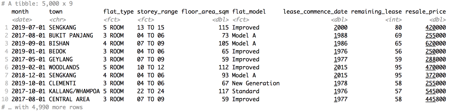
We will do this using a dataset of HDB resale flat prices. For now, we use a random sample of 3,000 transactions that occurred between Jan 2017 and Jan 2020 and will gradually bring in a larger version (~70k records in the last three years), as well as the geographic aspect (maps!) of this data. It is a nice dataset to work with since it is relatively clean (hurray!) and has a number of categorical and quantitative dimensions that, to derive insights from this data, benefit from visualization.

A single-view starting point

The original data can be download from the [data.gov.sg data portal]. I have pre-processed it in R and exported it directly to JSON. The original dataset contains about 70,000 sales records over the last 3 years. To speed up our initial experimentation, I have randomly selected 3,000 records out of this dataset. This is often a good idea in projects – it allows you to load and process data much faster. Once the project solidifies you can also swap in the original dataset. The R code for processing doesn't do anything fancy - just converting the variables to the right type and taking the sample. I'm including it below for your reference.

sales <- read_csv(here::here("data/hdb_resale_2017_onwards.csv")) %>% 
  mutate(month = ymd(month, truncated = 1),
         flat_type = as_factor(flat_type),
         storey_range = as_factor(storey_range),
         flat_model = as_factor(flat_model))

sales %>% 
  select(-block, -street_name) %>% 
  sample_n(3000) %>% 
  mutate(remaining_lease = substr(remaining_lease, 1, 2) %>% as.integer()) %>% 
  jsonlite::write_json(., "resale_sample_2017-2020.json")

The available variables in our dataset look like this:

Before we start to look at multiple aspects and variables at the same time, it is a good idea to do a quick sanity check to make sure the importing of our data goes OK. We will use the same pattern as in previous weeks, where we export const data = [... data goes ...] from a data.js file. We then import { data } from './data.js' in our App.svelte file.

I have already set this up for you in the below sandbox. In this sandbox, we follow the same procedure and pattern as last week to create a scatterplot of price (y axis) and floor area (x axis). This is a good pair of variables for a sanity check: we know that there should be a positive relationship between these two variables so we would certainly expect our graph to mirror that! The basic steps to create this graph are:

1. Importing our data.
2. Setting up two scales for the x and y axes – with appropriate domains for each variable.
3. Creating a Graph element with the appropriate properties (essentially: dimensions and scales)
4. Iterating over our dataset with {#each} to create a single Point element for each item in our data.

A tool for transforming data: the DataContainer

So far, we have used the provided data as-is. We import it and subsequently map it directly into a graphic representation without doing anything in terms of post-processing or transformation. However, for many visualizations – even something as simple as a histogram – we need to first transform and aggregate our data in different ways.

To make this process easier, florence has a sidecar library called DataContainer. It's already installed in the previous sandbox, but otherwise you can install it by running npm install @snlab/florence-datacontainer. To use it, import it in your project (import DataContainer from '@snlab/florence-datacontainer').

Once imported, we can convert our original data structure to a DataContainer, like so:

const sales = new DataContainer(data)

This sales DataContainer has a number of useful features – similar to a tibble in R's tidyverse or a DataFrame in Python's pandas. These features are implemented as methods or functions available on the DataContainer. We will start off with implementing the following two:

• DataContainer allows us to easily extract the domain for specific columns. This can be used to automatically calculate the correct scales for the x and y axis.
• DataContainer allows us to extract an entire column as a single Array. This is very useful because it allows us to use the PointLayer instead of a combination of the {#each} loop and the individual Point Marks, as we have done previously.

Facets

Until now, we have create a single view on our dataset inside of the Graphic. This isn't a necessity: we can include as many views as we'd like by using the 'Section'. You can think of the Section as allowing us to create different 'layers' for our visualization. These layers can be on 'top' of each other (so the have the same x/y properties) or next to each other (different x/y properties). For now, we are going to divide a Graphic into 4 equally sized sections. We will do so by manually setting the x1, x2, y1, and y2 properties of each Section to the appropriate pixel values. Later on, we will see how we can automate this procedure.

Data Transformations

The four coloured squares are placeholders for different facets of our HDB dataset. In this section, we will 'fill in' each square with the following visualizations:

• A bar chart showing the number of transactions per flat type
• A histogram showing the distribution of the resale price
• A scatterplot showing the relationship between price and floor area
• A line chart showing the development of resale price over time

To create each of these (except for #3 – that's a freebie), we will need to transform and aggregate the dataset in different ways. For this reason, DataContainer support a series of transformations that are heavily inspired by dplyr in R's tidyverse.

Let's get started on the first visualization together. To calculate the number of transactions per flat type, we can combine the group_by and summarise functions.

const salesPerType = sales
    .groupBy('flat_type')
    .summarise({ total_count: { resale_price: 'count' } })
console.log(salesPerType.data()) // we can check the results by writing out the entire table to the console (`.data()` prints the table in a legible format)

Once you have the data in the right structure, you think about how you map the data to the specific properties (i.e. 'channels' or 'aesthetics') of each Mark. In this case, let us put the categories of the flat_type on the y axis (scaleY) and the total_count on the x axis (scaleX). Our next steps consist of:

• We need to specify the appropriate scales. For total_count we can use the usual linear scale. But for flat_type we need a band scale.
• The x1 and x2 of the RectangleLayer will need to be determined by aspects of total_count. The y1 property will need to be determined by the flat_count. But to determine where the rectangle should stop (y2), we need to use both the flat_count and the bandwidth aspect of the scale. To do this, we specify the y2 not as a value in 'data space' but instead as a pre-calculated value in pixels. We can do this (on any Mark) by specifying a function rather than a number or string. Whatever value the function returns will be taken as the pixel position for that property. Importantly, the scales that belong to a section are available within the scope of that function and can be accessed through a process called object destructuring. You can see a simple example of this in Rectangle Mark docs.

Auto-generating facets

In the previous section, we have created 4 different sections or facets by hand. However, for larger systems this can become quite tedious. For this reason, florence has a built-in Grid component that allows you to construct both simple and more advanced ones. It largely follows the CSS Grid logic to do this.

Most importantly, you can specify a specific number of rows and columns -- and an optional list of area or cell names. The Grid will use this information to calculate the right positioning properties for any Sections within the Grid.

<Section {...cells[town]}>

<Section
 x1={cells[town].x1}
 x2={cells[town].x2}
 y1={cells[town].y1}
 y2={cells[town].y2}
>

Thursday class live-stream recording